Data Profiling using Matillion Grid Variables

Right across the industry, a consistent trend is that new data sources are constantly coming online, bringing new formats with them. Furthermore, all this new data keeps changing at an ever increasing rate.

But that doesn't mean automated data profiling has to be difficult! This article will demonstrate how to create a versatile data profiler by bringing together several Matillion DataOps technologies:

• Grid Variables, to flexibly handle metadata
• Transformation Jobs, to run data profiling efficiently
• A Shared Job wrapper, as a template for automation

The solution will be most relevant to anyone involved with DataOps or Data Quality. This article will also be useful alongside the Matillion Academy courses on Grid Variables, Shared Jobs and Python.

When data profiling is integrated with everyday activities of ingestion and transformation, it can be a great asset to productivity, and can help keep data quality high.

Prerequisites

The data profiler uses shared jobs and grid variables, so the only prerequisite is:

• Access to Matillion ETL

While reading this article, you may choose to look at the actual implementation yourself:

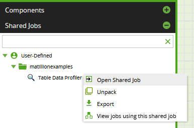
• Download and import the Table Data Profiler shared job from the Matillion Exchange
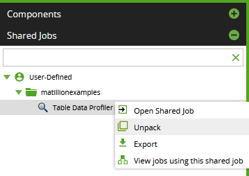
• While editing an Orchestration Job, go to the Shared Jobs panel, search for the Table Data Profiler, and from the context menu choose "Open Shared Job"

Data Profiling Tools

Data profiling requires a computation engine that can efficiently summarize large numbers of records. Also, the algorithms must be capable of handling diverse types of data.

The cloud data warehouse itself is the perfect place to do this work, for several reasons:

• Top performance - because the data is already in the right place
• Sophisticated - access to a range of inbuilt SQL functions created specifically for this type of analysis
• Cost effective and scalable - based on cloud economics

So, what does data profiling look like inside a database?

Data Profiling Examples

The simplest form of data profiling is to count the number of records in a table. The SQL expression is:

COUNT(*)

In the expression editor of a Matillion ETL Calculator component:

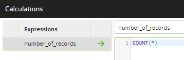
Even this basic profiling information can be powerful when captured regularly, since it can reveal trends in data volumes.

It's also easy to find out how many different values there are in one column:

COUNT(DISTINCT "column_name")

Now it's possible to combine those two figures. If the number of distinct values is equal to the number of records, then the column values are unique. This is a fundamental requirement for business identifiers like Data Vault hub tables.

Are any values missing? This involves summing an expression, for example:

SUM(CASE WHEN "column_name" IS NULL THEN 1 ELSE 0 END)

When a column has no missing values and they are all unique, then it is a valid primary key - and vice versa :-)

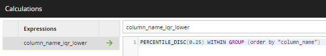
Lastly, something more sophisticated. For any numeric column, the interquartile range is a statistical property relevant to both dispersion and skew. The Snowflake SQL expression to find the 25th percentile (or "lower") IQR value is:

PERCENTILE_DISC(0.25) WITHIN GROUP (order by "column_name")

In Matillion ETL:

Your cloud data warehouse supports many more of these kinds of functions. It is often useful to combine the basic functions to arrive at more advanced calculations.

Building a data profiler that can handle any table will require much more than substituting one scalar variable for one column name. Entire lists of inter-related metadata will be needed. This is a job for Matillion grid variables.

Matillion Grid Variables

One grid variable is like a mini spreadsheet. Grid variables have named columns, and are defined inside a Matillion orchestration or transformation job. Many Matillion ETL components can be made metadata-driven thanks to tight integration with grid variables.

You can read and write to grid variables with dedicated components or using Python scripting. This data profiling example will use both techniques.

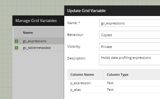
In the screenshot below, from the data profiling orchestration job, you can see there are two grid variables:

• gv_expressions - the SQL expressions for the data profiling metrics. Every expression will have an associated alias name
• gv_tablemetadata - all the column names and datatypes of the table being profiled. It also has two columns: col_name and col_type

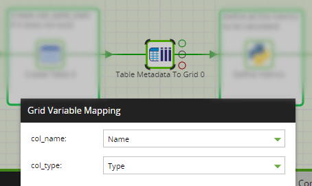
For a single database table, a Table Metadata To Grid component reads the column names and datatypes into gv_tablemetadata:

Now the job knows what columns are to be profiled, it can generate the necessary SQL statements. In Python, start with an empty list and add the expression/alias pairs by looping through the table metadata.

tabmeta = context.getGridVariable('gv_tablemetadata')

for c in tabmeta:

  alias = '"%s_distinct"' % (c[0])
  expr_list.append(['COUNT(DISTINCT "%s")' % (c[0]), alias])

You will recognize the SQL expression from the examples shown earlier. Notice how the column name is parameterized as col_name from gv_tablemetadata, which is c[0].

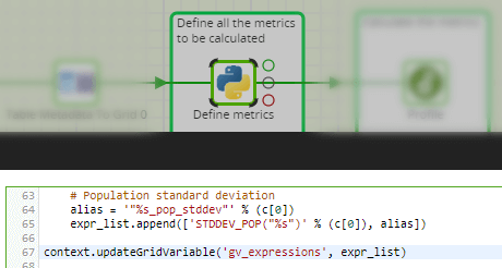
Many profiling expressions can be added for every column. Some are dependent on the datatype, c[1]. For example the standard deviation can only be calculated for numeric columns:

  if(isNumericDatatype(c[1])):
    alias = '"%s_pop_stddev"' % (c[0])
    expr_list.append(['STDDEV_POP("%s")' % (c[0]), alias])

The last step is to save all the dynamically generated SQL into gv_expressions:

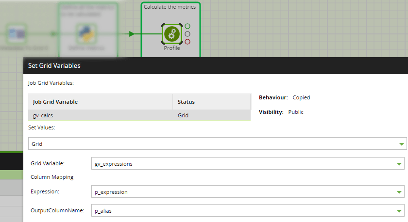
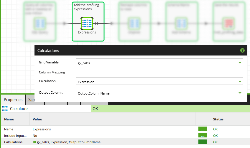
Evaluating all these SQL profiling expressions will be done by the cloud data warehouse. The Matillion ETL transformation job for this purpose has a waiting grid variable of its own, named gv_calcs. The Run Transformation component maps the columns of one grid variable onto the other:

Now the transformation job has the schema and table name, plus a list of all the data profiling expressions. It has become entirely metadata-driven.

Metadata Driven Data Transformation

The Matillion ETL transformation job that runs the data profiling uses several parameters expressed as public visibility job variables, including:

• Scalar variables tx_schema_name and tx_table_name
• The grid variable gv_calcs containing the SQL data profiling expressions alongside an alias name for each

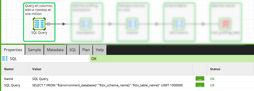
Data profiling begins by selecting rows from the table, using a SQL Script component shown below.

Note there is a rowstop limit of one million. This is optional - but for large tables, representative statistics can be obtained quickly just by sampling.

Next there is a Calculator component in grid variable mode. This is where the metadata from gv_calcs is injected. It creates a single large SQL statement for the cloud data warehouse to execute.

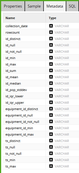
Output from the Calculator is a "wide" table: just one row, with one column for every single metric. As an example, below is the output from profiling the norm_bubble_event table in the preinstalled example jobs.

The information is great, but it needs to be transposed into a schema-neutral format. This is done with an UNPIVOT in the following SQL component.

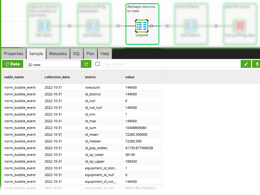
Now the profiling data is resistant to schema drift. Tables and columns may come and go, but the schema for the metrics stays constant.

The last components in the job add the schema name and append the profiling data into a database table named metl_profiling_data.

So far I have been deliberately diving into the details to show how the job works. In a production environment it would be better to encapsulate all that and expose only a schema and table name as parameters. Matillion has Shared Jobs for this purpose.

Building a Shared Job

Matillion Shared Jobs always start with one Orchestration Job. This is known as the entry point or "root" job. All its public visibility parameters become the component properties of the Shared Job.

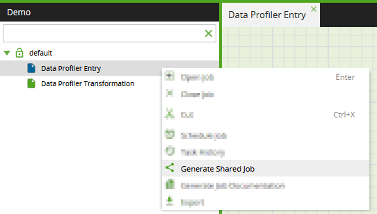
When you are satisfied the parameters in the root job are working, choose Generate Shared Job from a context click in the folder structure.

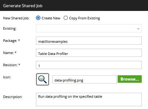
In the popup dialog, use your company name in the package name. This will differentiate it from all the built-in shared jobs.

Choose a name, revision and description, and select an icon. Small, square PNG images work well.

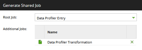
The dialog will detect if other jobs need to be included. In this case there is one additional transformation job:

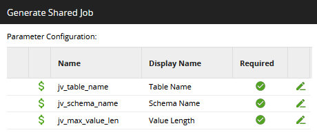
Give the parameters more friendly display names:

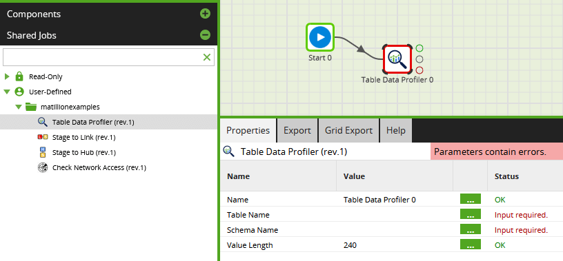
Once the new Shared Job has been generated, you can use it in any orchestration job by dragging it in from the sidebar.

Notice how the public visibility parameters appear as individual properties of the Shared Job, complete with their friendly display names.

Now your data profiling can be automated! You can run this shared job inside an iterator to profile all your database tables.

Next Steps

Add the data profiling metrics that are most relevant for your data, taking advantage of all the aggregate SQL functions that are available inside your cloud data warehouse.

To make your own copy of a Shared Job, choose Unpack from the context menu. This creates local copies of the embedded Jobs, that you can edit and repackage.

Operationalize data profiling into your Matillion ETL workflows: gather history, and watch for trends. It is likely that the profiling data will have a relationship with any job performance tuning data you are capturing.

Take the Matillion Academy courses on Grid Variables, Shared Jobs and Python.