- Blog
- 01.11.2022
Data Warehouse Time Variance with Matillion ETL

Building and maintaining a cloud data warehouse is an excellent way to help obtain value from your data. A couple of very common examples are:
- The data warehouse provides a single, consistent view of historical operations. This is the foundation for measuring KPIs and KRs, and for spotting trends
- The data warehouse provides a reliable and integrated source of facts. This means it can be used to feed into correlation and prediction machine learning algorithms
The ability to support both those things means that the Data Warehouse needs to know when every item of data was recorded. This is the essence of time variance.
In this article, I will run through some ways to manage time variance in a cloud data warehouse, starting with a simple example.
Aligning past customer activity with current operational data
Let’s say we had a customer who lived at Bennelong Point, Sydney NSW 2000, Australia, and who bought products from us. In 2020 they moved to Tower Bridge Rd, London SE1 2UP, United Kingdom, and continued to buy products from us.
Most operational systems go to great lengths to keep data accurate and up to date. In this example, to minimise the risk of accidentally sending correspondence to the wrong address.
So if data from the operational system was used to assess the effectiveness of a 2019 marketing campaign, the analyst would probably be scratching their head wondering why a customer in the United Kingdom responded to a marketing campaign that targeted Australian residents.
Analysis done that way would be inaccurate, and could lead to false conclusions and bad business decisions.
The root cause is that operational systems are mostly not time variant. For reasons including performance, accuracy, and legal compliance, operational systems tend to keep only the latest, current values. Old data is simply overwritten.
In the next section I will show what time variant data structures look like when you are using Matillion ETL to build a data warehouse.
Time variant data structures
Time variance means that the data warehouse also records the timestamp of data. So inside a data warehouse, a time variant table can be structured almost exactly the same as the source table, but with the addition of a timestamp column.
Here is a simple example:
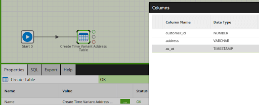
The extra timestamp column is often named something like “as-at”, reflecting the fact that the customer’s address was recorded as at some point in time.
There are several common ways to set an as-at timestamp.
- If there is auditing or some form of history retention at source, then you may be able to get hold of the exact timestamp of the change according to the operational system. There is more on this subject in the next section under “Type 4” dimensions.
- A change data capture (CDC) process should include the timestamp when CDC detected the change
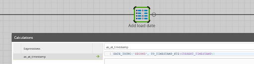
- During the extract and load, you can record the timestamp when the data warehouse was notified of the change. A Calculator component in a Transformation Job is a good way, for example like this:
Once an as-at timestamp has been added, the table becomes time variant. It is capable of recording change over time. The data can then be used for all those things I mentioned at the start: to calculate KPIs, KRs, look for historical trending, or feed into correlation and prediction algorithms.
Here is a screenshot of simple time variant data in Matillion ETL:
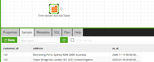
As the screenshot shows, one extra as-at timestamp really is all you need. In a more realistic example, there are more sophisticated options to consider when designing a time variant table:
- It is very useful to add a unique key column on every time variant data warehouse table. This is usually numeric, often known as a surrogate key, and can be generated for example from a sequence. Alternatively, in a Data Vault model, the value would be generated using a hash function. The next section contains an example of how a unique key column like this can be used.
- The surrogate key can be made subject to a uniqueness or primary key constraint at the database level
- You may choose to add further unique constraints to the database table. In the example above, the combination of customer_id plus as_at should always be unique. That way it is never possible for a customer to have multiple “current” addresses.
- Check what time zone you are using for the as-at column. A good solution is to convert to a standardized time zone according to a business rule.
However, adding extra time variance fields does come at the expense of making the data slightly more difficult to query.
For example, why does the table contain two addresses for the same customer? Well, it’s because their address has changed over time. If you want to know the correct address, you need to additionally specify when you are asking.
For end users, it would be a pain to have to remember to always add the as-at criteria to all the time variant tables. Furthermore, in SQL it is difficult to search for the “latest record before this time”, or the “earliest record after this time”.
So to achieve gold standard consumability, time variance is usually represented in a slightly different way in a presentation layer such as a star schema data model. In that context, time variance is known as a slowly changing dimension.
Slowly Changing Dimensions
A data warehouse presentation area is usually modeled as a star schema, and contains dimension tables and fact tables. Much of the work of time variance is handled by the dimensions, because they form the link between the transactional data in the fact tables.
To continue the marketing example I have been using, there might be one fact table: sales, and two dimensions: campaigns and customers. To keep it simple, I have included the address information inside the customer dimension (which would be an unusual design decision to make for real). Also, normal best practice would be to split out the fields into the address lines, the zip code, and the country code.
Exactly like the time variant address table in the earlier screenshot, a customer dimension would contain two records for this person, for example like this:
| Surrogate key | Business key | Address | Valid from | Valid to | |||||
|---|---|---|---|---|---|---|---|---|---|
| 21937 | 123 | Bennelong Point, Sydney NSW 2000, Australia | 2000-11-14 | 2020-01-28 | |||||
| 1445745 | 123 | Tower Bridge Rd, London SE1 2UP, United Kingdom | 2020-01-29 |
Important details to notice:
- This kind of structure is known as a “slowly changing dimension”. Not that there is anything particularly “slow” about it. Focus instead on the way it records changes over time. A more accurate term might have been just a “changing dimension.”
- All of the historical address changes have been recorded.
- This particular representation, with historical rows plus validity ranges, is known as a “Type 2” slowly changing dimension. Type 2 is the most widely used, but I will describe some of the other variations later in this section.
- The business key is meaningful to the original operational system. In this case it is just a copy of the customer_id column. This is how to tell that both records are for the same customer
- The surrogate key is subject to a primary key database constraint. It is guaranteed to be unique. This makes it a good choice as a foreign key link from fact tables.
- The surrogate key has no relationship with the business key. It is impossible to work out one given the other.
- The Valid From and Valid To dates make ranges of validity. Data warehouse transformation processing ensures the ranges do not overlap. In this example they are day ranges, but you can choose your own granularity such as hour, second, or millisecond. As an alternative, you could choose to make the prior Valid To date equal to the next Valid From date.
- The last (i.e. current) record has no Valid To value. As an alternative you could choose to use a fixed date far in the future.
We have been making sales to this customer for many years: before and after their change of address. So the sales fact table might contain the following records:
| Date | Sale amount | Campaign ID | Customer ID | ||||||||
|---|---|---|---|---|---|---|---|---|---|---|---|
| 2019-04-21 | $100 | Aus1 | 21937 | ||||||||
| 2019-08-01 | $40 | Aus1 | 21937 | ||||||||
| 2020-08-30 | $160 | 1445745 |
Notice the foreign key in the Customer ID column points to the surrogate key in the dimension table. This is how the data warehouse differentiates between the different addresses of a single customer.
Now a marketing campaign assessment based on this data would make sense:
- The analyst can tell from the dimension’s business key that all three rows are for the same customer. They would attribute total sales of $300 to customer 123.
- The analyst would also be able to correctly allocate only the first two rows, or $140, to the Aus1 campaign in Australia. Because it is linked to a time variant dimension, the sales are assigned to the correct address as at the time every sale was made.
The customer dimension table above is an example of a “Type 2” slowly changing dimension. It records the history of changes, each version represented by one row and uniquely identified by a time/date range of validity.
Some other attributes you might consider adding to a Type 2 slowly changing dimension are:
- A “latest” flag – a boolean value, set to TRUE for the latest record for every business key, and FALSE for all the earlier records. This makes it very easy to pick out only the current state of all records.
- Version number – an ascending integer.
- A hash code generated from all the “value” columns in the dimension – useful to quickly check if any attribute has changed.
- If the concept of deletion is supported by the source operational system, a logical deletion flag is a useful addition. You cannot simply delete all the values with that business key because it did exist as at times in the past. A physical CDC source is usually helpful for detecting and managing deletions.
As you would expect from its name, “Type 2” is not the only way to represent time variance in a dimension table…
Type 1
This option does not implement time variance. Instead it just shows the latest value of every dimension, just like an operational system would. The advantages are that it is very simple and quick to access.
| Surrogate key | Business key | Address | ||||||
|---|---|---|---|---|---|---|---|---|
| 1445745 | 123 | Tower Bridge Rd, London SE1 2UP, United Kingdom |
Some important features of a Type 1 dimension are:
- The surrogate key is an alternative primary key. It is most useful when the business key contains multiple columns.
- There is no way to discover previous data values from a Type 1 dimension. The historical data either does not get recorded, or else gets overwritten whenever anything changes. There is no “as-at” information.
Type 2
The main example I used at the start of this section was a Type 2. There can be multiple rows for the same business entity, each row containing a set of attributes that were correct during a date/time range.
A business decision always needs to be made whether or not a particular attribute change is significant enough to be recorded as part of the history. As an example, imagine that the question of whether a customer was “in office hours” or “outside office hours” was important at the time of a sale. Office hours are a property of the individual customer, so it would be possible to add an “inside office hours” boolean attribute to the customer dimension table.
But the value will change at least twice per day, and tracking all those changes could quickly lead to a wasteful accumulation of almost-identical records in the customer table. A better choice would be to model the “in office hours” attribute in a different way, such as on the fact table, or as a Type 4 dimension.
Type 3
A Type 3 dimension is very similar to a Type 2, except with additional column(s) holding the previous values. With this approach, it is very easy to find the prior address of every customer.
| Surrogate key | Business key | Address | Prior address |
|---|---|---|---|
| 21937 | 123 | Bennelong Point, Sydney NSW 2000, Australia | |
| 1445745 | 123 | Tower Bridge Rd, London SE1 2UP, United Kingdom | Bennelong Point, Sydney NSW 2000, Australia |
Aside from time variance, the type 3 dimension modeling approach is also a useful way to maintain multiple alternative views of reality. An example might be the ability to easily flip between viewing sales by “new” and “old” district boundaries.
Type 4
There are different interpretations of this, usually meaning that a Type 4 slowly changing dimension is implemented in multiple tables.
A widely used approach is to have:
- One “current” table, equivalent to a Type 1 dimension.
- One “historical” table that contains all the older values. The historical table contains a timestamp for every row, so it is time variant.
This kind of structure is rare in data warehouses, and is more commonly implemented in operational systems. The current table is quick to access, and the historical table provides the auditing and history. One task that is often required during a data warehouse initial load is to find the “historical” table. Data from there is loaded alongside the current values into a single time variant dimension.
Another widely used Type 4 approach is to split a single dimension into more than one table, based on the frequency of updates. Referring back to the “office hours” question I mentioned a few paragraphs ago, a solution might be to separate that volatile attribute into a new, compact dimension containing only two values: true and false.
Type 5
Similar to the previous case, there are different “Type 5” interpretations. The most common one is when rapidly changing attributes of a dimension are artificially split out into a new, separate dimension, and the dimensions themselves are linked with a foreign key.
Type 6
A Type 6 dimension is very similar to a Type 2, except with aspects of Type 1 and Type 3 added. There are new column(s) on every row that show the current value.
| Surrogate key | Business key | Address | Current address |
|---|---|---|---|
| 21937 | 123 | Bennelong Point, Sydney NSW 2000, Australia | Tower Bridge Rd, London SE1 2UP, United Kingdom |
| 1445745 | 123 | Tower Bridge Rd, London SE1 2UP, United Kingdom | Tower Bridge Rd, London SE1 2UP, United Kingdom |
This is very similar to a Type 2 structure. The main advantage is that the consumer can easily switch between the current and historical views of reality.
Physical time variance implementation
In this section, I will walk though a way to maintain a Type 1 and a Type 2 dimension using Matillion ETL. I will be describing a physical implementation: in other words, a real database table containing the dimension data. This type of implementation is most suited to a two-tier data architecture.
For a Type 1 dimension update, there are two important transformations:
- A Table Update Component that
- inserts any values that are not present yet
- updates any values that have changed
- Matillion will attempt to run an SQL update statement using a primary key (the business key), so it’s important to deduplicate the incoming data.
So in Matillion ETL, a Type 1 update transformation might look like this:
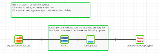
In the above example I do not trust the input to not contain duplicates, so the rank-and-filter combination removes any that are present. The Table Update component at the end performs the inserts and updates.
As you would expect, maintaining a Type 1 dimension is a simple and routine operation. As an alternative to creating the transformation yourself, a logical CDC connector can automate it.
Maintaining a physical Type 2 dimension is a quantum leap in complexity. It begins identically to a Type 1 update, because we need to discover which records – if any – have changed. Matillion has a Detect Changes component for exactly this purpose.
The Detect Changes component requires two inputs:
- The new data that has just been extracted and loaded, and deduplicated
- The current data from the dimension
New data must only be compared against the current values in the dimension, so a filter is needed on that branch of the data transformation:
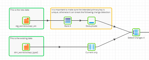
The Detect Changes component adds a flag to every new record, with the value ‘C’, ‘D’, ‘I’ or ‘N’ depending if the record has been Changed, Deleted, or if it is Identical or New.
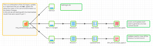
It is important not to update the dimension table in this Transformation Job. It may be implemented as multiple physical SQL statements that occur in a non deterministic order. Instead, save the result to an intermediate table and drive the database updates from that intermediate table in a second transformation.
The second transformation branches based on the flag output by the Detect Changes component. This is based on the principle of complementary filters.
- For records that are Identical, no action is necessary.
- For records that are either New or Changed, a new record is always needed to store the current value. So that branch ends in a Table Output Component in append mode.
- For records that are Changed, there is an older record that needs to be closed. Its validity range must end at exactly the point where the new record starts. So that branch ends in a Table Update Component with the insert mode switched off. Only the “Valid To” date and the “Current Flag” need to be updated.
In Matillion ETL the second Transformation Job could look like this:
It is vital to run the two Transformation Jobs in the correct order. It is also desirable to run all dimension updates near in time to each other, so that the entire data warehouse represents a single point in time as nearly as possible.
It is clear that maintaining a single Type 2 slowly changing dimension is much more demanding than a Type 1, requiring around 20 transformation components. Even more sophistication would be needed to handle the extra work for Types 3, 4, 5 and 6.
Furthermore, the jobs I have shown above do not handle some of the more complex circumstances that occur fairly regularly in data warehousing. Examples include:
- Out-of-sequence updates – Manual updates are sometimes needed to handle those cases, which creates a risk of data corruption.
- Deletion of records at source – Often handled by adding an “is deleted” flag. Technically that is fine, but consumers then always need to remember to add it to their filters.
- Changes to the business decision of what columns are important enough to register as distinct historical changes – Once that decision has been made in a physical dimension, it cannot be reversed. Historical changes to “unimportant” attributes are not recorded, and are lost.
Any time there are multiple copies of the same data, it introduces an opportunity for the copies to become out of step. To minimize this risk, a good solution is to look at virtualizing the presentation layer star schema.
Virtualized time variance implementation
First, a quick recap of the data I showed at the start of the “Time variant data structures” section earlier: a table containing the past and present addresses of one customer.
The table has a timestamp, so it is time variant. In fact, any time variant table structure can be generalized as follows:
- A business key that uniquely identifies the entity, such as a customer ID
- Attributes – all the properties of the entity, such as the address fields
- An as-at timestamp containing the date and time when the attributes were known to be correct
This combination of attribute types is typical of the Third Normal Form or Data Vault area in a data warehouse. Alternatively, tables like these may be created in an Operational Data Store by a CDC process. There is enough information to generate all the different types of slowly changing dimensions through virtualization.
A Type 1 dimension contains only the latest record for every business key. This can easily be picked out using a ROW_NUMBER analytic function, implemented in Matillion by the Rank component followed by a Filter.
With virtualization, a Type 2 dimension is actually simpler than a Type 1! No filtering is needed, and all the time variance attributes can be derived with analytic functions.
- Valid from – this is just the as-at timestamp
- Valid to – using a LEAD function to find the next as-at timestamp, subtract 1 second
- Latest flag – true if a ROW_NUMBER function ordering by descending as-at timestamp evaluates to 1, otherwise false
- Version number – using another ROW_NUMBER function ordering by the as-at timestamp ascending
Joining any time variant dimension to a fact table requires a primary key. It is very helpful if the underlying source table already contains such a column, and it simply becomes the surrogate key of the dimension.
Continuing to a Type 3 slowly changing dimension, it is the same as a Type 2 but with additional prior values for all the attributes. These can be calculated in Matillion using a Lead/Lag Component.
Below is an example of how all those virtual dimensions can be maintained in a single Matillion Transformation Job:
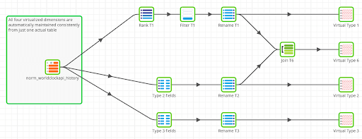
Even the complex Type 6 dimension is quite simple to implement. When virtualized, a Type 6 dimension is just a join between the Type 1 and the Type 2.
Business users often waver between asking for different kinds of time variant dimensions. When you ask about retaining history, the answer is naturally always yes. But later when you ask for feedback on the Type 2 (or higher) dimension you delivered, the answer is often a wish for the simplicity of a Type 1 with no history.
If you choose the flexibility of virtualizing the dimensions, there is no need to commit to one approach over another. You can implement all the types of slowly changing dimensions from a single source, in a declarative way that guarantees they will always be consistent.
Virtualizing the dimensions in a star schema presentation layer is most suitable with a three-tier data architecture.
Time variance recap and summary
A “time variant” table records change over time. The only mandatory feature is that the items of data are timestamped, so that you know when the data was measured.
The very simplest way to implement time variance is to add one as-at timestamp field. But to make it easier to consume, it is usually preferable to represent the same information as a valid-from and valid-to time range. Typically that conversion is done in the formatting change between the Normalized or Data Vault layer and the presentation layer.
It is possible to maintain physical time variant dimensions with valid-from and valid-to timestamps, and a range of other useful attributes. However, this tends to require complex updates, and introduces the risk of the tables becoming inconsistent or logically corrupt. For those reasons, it is often preferable to present virtualized time variant dimensions, usually with database views or materialized views.
The advantages of this kind of virtualization include the following:
- Virtualization reduces the complexity of implementation
- Virtualization removes the risk of physical tables becoming out of step with each other. The same thing applies to the risk of the individual time variance attributes becoming inconsistent.
- Virtualization is a declarative solution rather than imperative. The “updates” are always immediate, fully in parallel and are guaranteed to remain consistent.
- It is easy to implement multiple different kinds of time variant dimensions from a single source, giving consumers the flexibility to decide which they prefer to use.
- Historical updates are handled with no extra effort or risk
- The business decision of which attributes are important enough to be history tracked is reversible. The underlying time variant table contains all the changes.
- Virtualized dimensions do not consume any space
Time is one of a small number of universal correlation attributes that apply to almost all kinds of data. Another example is the geospatial location of an event.
Time variance is a consequence of a deeper data warehouse feature: non-volatility. Operational systems often go out of their way to overwrite old data in an effort to stay accurate and up to date, and to deliver optimal performance. But in doing so, operational data loses much of its ability to monitor trends, find correlations and to drive predictive analytics. This is one area where a well designed data warehouse can be uniquely valuable to any business.
See how Matillion ETL can help you build time variant data structures and data models
You can try all the examples from this article in your own Matillion ETL instance.
To install the examples, log into the Matillion Exchange and search for the Developer Relations Examples Installer:
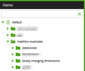
Follow the instructions to install the example jobs. You will find them in the “slowly changing dimensions” folder under “matillion-examples”.
And to see more of what Matillion ETL can help you do with your data, get a demo.
Featured Resources
VMware and AWS Alumnus Appointed Matillion Chief Revenue Officer
Data integration firm adds cloud veteran Eric Benson to drive ...
BlogHow Matillion Addresses Data Virtualization
This blog is in direct response to the following quote from ...
BlogMastering Git at Matillion. Exploring Common Branching Strategies
Git-Flow is a robust branching model designed to streamline the development workflow. This strategy revolves around two main ...
Share: